LIFE PROCESSES - ANIMAL PHYSIOLOGY
CLASS PRACTICAL RESULTS
There were consistent differences between NH3 excretion rates of crayfish fed on potato and bloodworm in all classes. Results are shown as mean ± standard deviation (a measure of the variability of the data) and sample size n (the number of pairs of students reporting data) in Table 1.
Table 1. Rate of NH3 excretion (μmol g-1 h-1) on two diets
| Class | Potato | Bloodworm | n | P |
| 1 | 0.084 ± 0.046 | 0.144 ± 0.056 | 9 | 0.027 |
| 2 | 0.097 ± 0.058 | 0.172 ± 0.077 | 11 | 0.019 |
| 3 | 0.105 ± 0.062 | 0.176 ± 0.106 | 11 | 0.071 |
| 4 | 0.090 ± 0.058 | 0.171 ± 0.122 | 11 | 0.062 |
| 5 | 0.063 ± 0.054 | 0.145 ± 0.137 | 11 | 0.080 |
| 6 | 0.112 ± 0.054 | 0.165 ± 0.042 | 9 | 0.034 |
Results of a t test comparing the two diets are also shown for each class. You may be familiar with this test for two samples of a measured variable. The P value shows the probability that the true NH3 excretion rates were the same for the two diets, with the two samples just differing by chance. The P values were less than 0.05 for classes 1, 2 & 6, which is usually taken as the criterion for a statistically significant result. In other words, we would conclude that the difference in NH3 excretion between potato and bloodworm diets observed in these classes was real. Results for classes 3-5 were similar, but not significant, largely due to the greater variability of the bloodworm data on those days.
We can combine the data from all classes in an analysis of variance (ANOVA). This statistical method is similar to the t test but can compare more than 2 samples, and make comparisons along more than one axis. Results of two-way ANOVA of NH3 excretion rates by diet and class are shown in Table 2.
Table 2. Two-way ANOVA of rate of NH3 excretion by diet and class
| P | |
| Diet | <0.001 |
| Class | 0.632 |
| Diet x Class | 0.991 |
The first row shows the probability that the true NH3 excretion rates were the same for the two diets, with differences just being due to chance. The P value is very low, and is regarded as statistically highly significant. The second row shows the probability that differences between NH3 excretion rates observed in different classes were due to chance. This P value is high, well over 0.05, so we conclude that there were no significant differences between the rates observed by different classes. The third row shows the interaction between diet and class, which also has a very high P value. This interaction is rather advanced statistics, but basically shows that the difference between the two diets was the same for each class.
We can conclude that there was a real difference in NH3 excretion rates between crayfish fed potato and bloodworm diets. The overall means were 0.091 μmol g-1 h-1 for the potato diet and 0.163 μmol g-1 h-1 for the bloodworm diet.
Your write-up should note any modifications to the methods described on the schedule and the reasons for these, and your own measurements (including a graph of the standard curve) and the calculations made from these. You can then use the overall means to discuss the effect of diet on NH3 excretion rates, and answer the questions given on the schedule.
Attach a graph of the absorption spectra of oxyhaemoglobin and deoxyhaemoglobin of rat blood to your report, and write a paragraph to answer the questions on the schedule. Note that "other animals" does not mean other mammals - spectra for other species of mammal will be almost identical.
Our results were expressed as mass-specific (i.e. per gram of fish) oxygen consumption. You will need to distinguish this clearly from the total oxygen consumption (i.e. per fish) when thinking about the results and comparing them with patterns from textbooks.
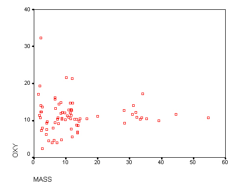
MO2 of the goldfish in relation to body mass is shown in Fig. 1 below. The large fish gave consistent results, but the small fish were highly variable. Some small fish had higher mass-specific MO2 than larger fish, others had lower mass-specific MO2 than larger fish. These results were tested using another analysis of variance, a one-way ANOVA of mass-specific oxygen consumption between the classes, with body mass as a covariate (i.e. a continuous variable, rather than a category such as class or diet), as shown in Table 3.
Figure 1. Graph of oxygen consumption (mmol g-1 h-1) on body mass (g)
Table 3. ANOVA of O2 consumption (mmol g-1 h-1) by class, with body mass covariate
| P | |
| Class | 0.306 |
| Mass | 0.948 |
There was no significant difference between the six classes, and no effect of body mass on mass-specific oxygen consumption. We will therefore use a data set from last year to examine the effect of body size on oxygen consumption in goldfish, in Table 4.
Table 4. Previous class data on mass-specific oxygen consumption and body mass
| Mass (g) | 10 | 30 | 15 | 40 | 7 | 60 | 10 | 30 | 15 | 12 | 15 | 5 | 50 | 2 |
MO2 (mmol g-1 h-1) | 23.7 | 7.4 | 10.7 | 7.5 | 27.6 | 3.0 | 22.9 | 8.8 | 6.4 | 12.2 | 19.2 | 9.0 | 5.2 | 25.2 |
| Mass (g) | 7 | 15 | 4 | 15 | 5 | 15 | 45 | 15 | 15 | 20 | 2 | 65 | 50 | 5 |
MO2 (mmol g-1 h-1) | 19.0 | 6.2 | 33.9 | 8.3 | 16.1 | 2.5 | 2.2 | 13.6 | 19.9 | 13.9 | 25.7 | 3.4 | 4.3 | 39.6 |
The relationship between mass-specific oxygen consumption and body mass in this data set is highly significant (P<0.001).
Your write-up should note any modifications to the methods described on the schedule and the reasons for these, and your own measurements and the calculations made from these. Plot ventilation rates of the experimental and control fish and answer the questions on the schedule. You can then use the data from last year to discuss the effect of body mass on oxygen consumption. Plot a graph of MO2 against log mass and answer the questions on the schedule - there is no need for further statistical analysis. Can you think of any explanations for the pattern in our own goldfish data?